Final Report
Introduction
Diabetes is a metabolic disorder that causes high blood glucose levels which might lead to health complications, including heart disease, stroke, kidney disease, and blindness. Since early detection is crucial to prevent complications machine learning models have been used to identify individuals at high risk based on demographic, lifestyle, and clinical data. This project aims to aid healthcare professionals in taking preventive measures to manage diabetes.
Project Statement
We aim to evaluate supervised learning algorithms for diabetes prediction. We will compare the performance on both the original dataset and a reduced-dimension dataset to identify significant risk factors to predict the disease. This can help design shorter surveys to only obtain information about these risk factors.
Data Collection
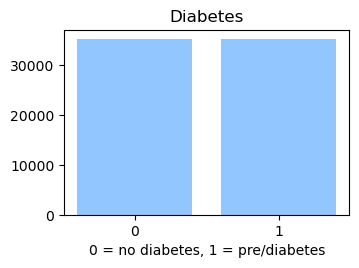
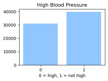
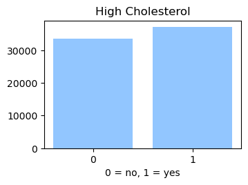
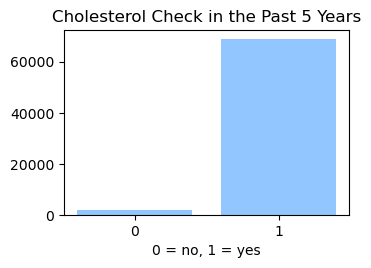
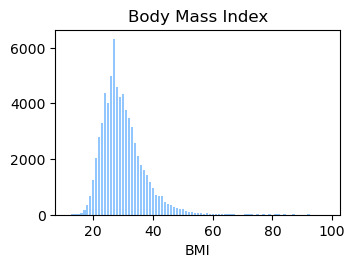
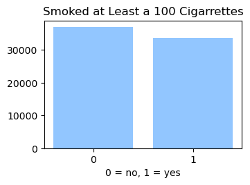
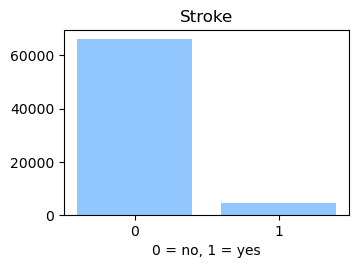
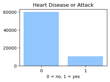
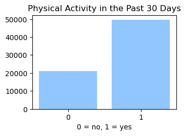
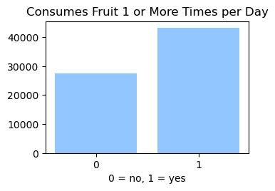
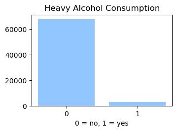
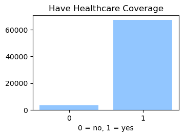
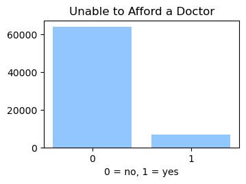
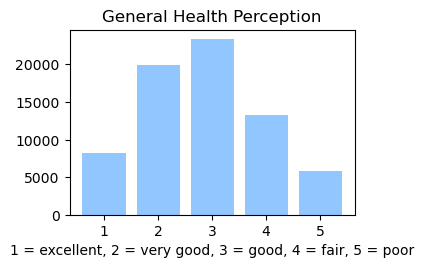
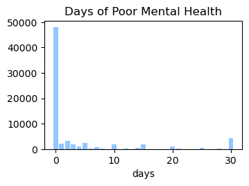
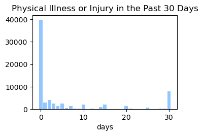
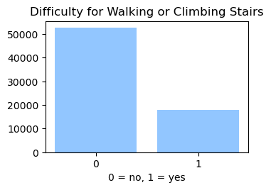
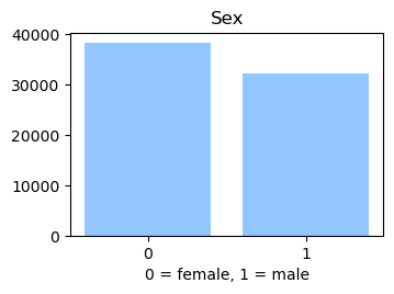
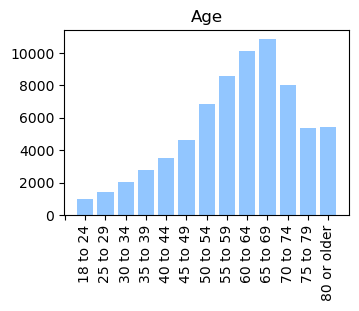
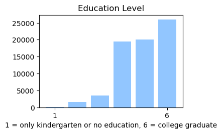
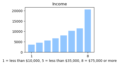
We used the Diabetes Health Indicator Dataset(1) which is a cleaned version of the 2015 Behavioral Risk Surveillance System Survey(2). The main file has 70,692 data points and 21 feature variables with a class balance for the labels. In addition, the dataset includes two more files with 253,680 data points and 21 feature variables with class imbalance. Below we present the frequencies of each of the dataset's features.

Methods
Supervised Learning
We predicted if a person has diabetes or not based on the health indicator features in the dataset. Choubey et al(3) have utilized methods like Logistic regression, K-nearest neighbor, Naïve Bayes, and Decision trees. Hasan et al(4) have used K-nearest neighbor, Naïve Bayes, Decision trees, Random Forest, AdaBoost, XGBoost, and an ensemble model to predict diabetes. Both papers use the Pima Indian Diabetic Dataset(5) which has 768 data points and 8 features. Choubey et al(3) also use the Localized Diabetes Dataset which has 1058 data points and 12 features. We applied the classification methods – Logistic Regression, K-nearest neighbor,Naïve Bayes, and Support Vector Machines on our Diabetes Health Indicator Dataset (1) and evaluated the performance of these models.
Unsupervised Learning
We employed Principal Component Analysis (PCA) as a dimensionality reduction technique for our dataset, with the expectation that our supervised learning models might exhibit better performance when applied to the reduced data(3). Consequently, we aim to assess the performance of our models using both the original dataset and the dataset transformed by PCA. This comparative evaluation will help us determine the effectiveness of PCA in improving our models' performance.
Results and Discussion
Data Analysis and Preprocessing
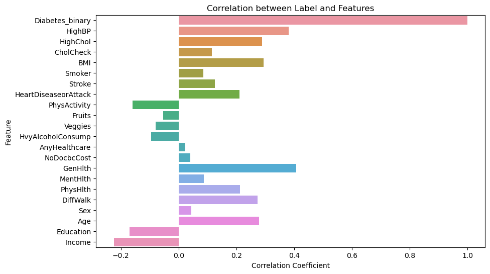
In the Data Collection section, we generated visualizations to gain a deeper understanding of our dataset. We found that our data is categorical and requires normalization, as the features have different scales. Furthermore, we calculated the correlation between the label column (indicating whether a person has diabetes) and all other features. The figure below shows that the features exhibit weak to moderate correlations with the label column.
Before applying any machine learning models, we preprocessed the data. The dataset was already clean, with no missing values and numeric scales. Consequently, we divided the dataset into an 80% training set and a 20% test set. We then fitted a MinMax scaler from the scikit-learn library to the training data, using it to normalize both the training and test sets. Afterward, we created new CSV files containing both datasets with the help of the Pandas library.
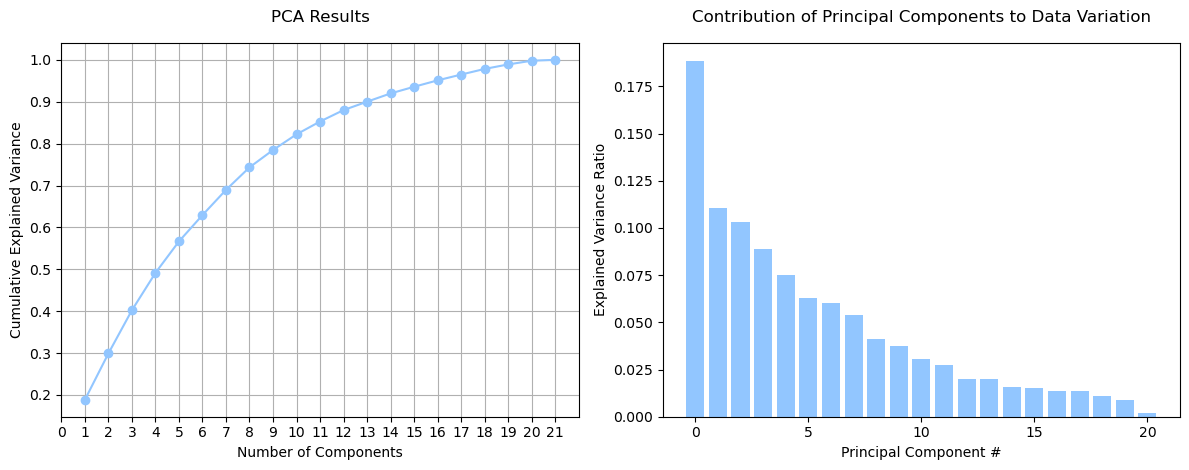
We used these training and test sets for all supervised learning models presented in this midterm report. Additionally, we employed Principal Component Analysis (PCA) to assess whether dimensionality reduction could lead to better model performance with less information. We performed PCA on our 21 features (excluding the label column) using the scikit-learn library and set a random state of 42 to ensure consistent results across multiple runs. Next, we calculated the explained variance ratio and the cumulative explained variance for each principal component. As depicted in the figure below, no single principal component accounts for the majority of data variation, with 13 principal components required to reach 90% of the variation.
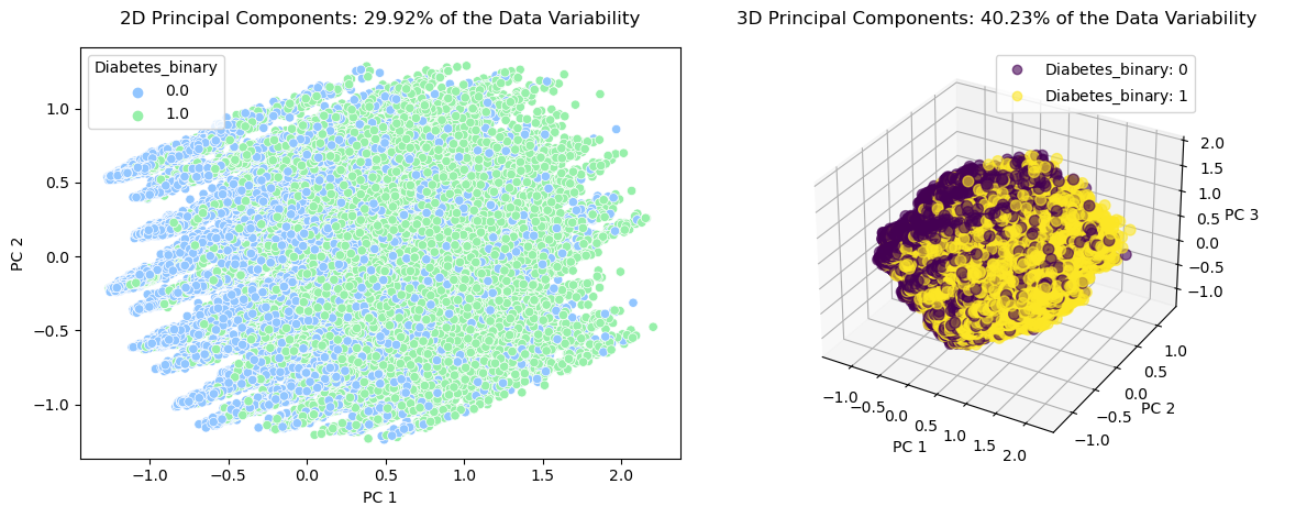
We plotted the data using two and three principal components, which accounted for 29.9% and 40.23% of the data's variation, respectively. However, identifying clusters or relationships within the data proved difficult due to the limited representation of data variation. The figure below displays the classified data, where label 0 represents no diabetes and label 1 represents diabetes.
We decided against applying clustering algorithms since two or three principal components inadequately represented the data's variation. Nevertheless, we performed PCA to obtain 13 and 16 principal components, which account for 90% and 95% of the data's variation, respectively. Our goal is to use these principal components to train our models and evaluate whether we can achieve better performance without relying on 21 dimensions. This work will be carried out for our final report.
Logistic Regression
The logistic regression model was trained using the train set and evaluated on the test set, which contained 14,139 data points. Both L1 norm (Lasso regression) and L2 norm (Ridge regression) yielded similar results in terms of model performance.
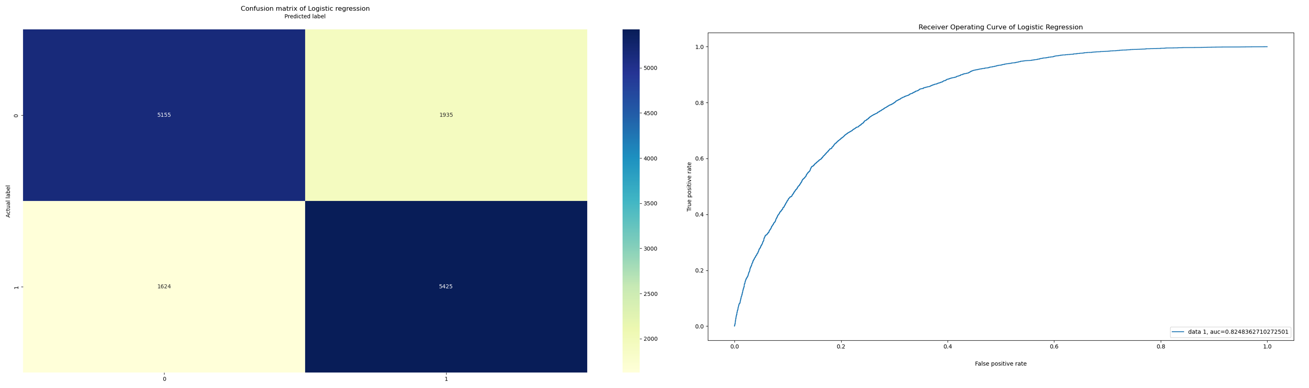
Despite adjusting various parameters, such as the solver, regularization strength, and class weight, there were no significant differences in the results. We then employed logistic regression with cross-validation (CV) to optimize the hyperparameters. However, altering the number of folds in the cross-validation process did not lead to any notable improvements in the model's performance. Across all cases, the model achieved an accuracy of 0.748, with a precision of 0.76 for class 0' (no diabetes) and 0.74 for class '1' (diabetes/pre-diabetes).
The logistic regression algorithm's performance was average, with a 75% accuracy rate. Therefore, we trained the model using PCA reduced datasets, where 95% and 90% of the explained variance was retained expecting to obtain a better perfomance. Nonetheless, the resulting accuracies were 72.5% and 72.3%, respectively.
To find if a different feature selection strategy could help us improving the model's perfomance we used forward feature selection on the training set utilizing the mlxtend library. Initially, the k-features parameter was set to 'best' to choose the feature subset with the highest cross-validation performance for 5-fold cross-validation. The forward feature selector chose 16 features: ['HighBP', 'HighChol', 'CholCheck', 'BMI', 'Stroke', 'HeartDiseaseorAttack', 'HvyAlcoholConsump', 'AnyHealthCare', 'NoDocbcCost', 'GenHlth', 'MentHlth', 'PhysHlth', 'DiffWalk', 'Sex', 'Age', 'income']. With these features, a logistic regression model was trained and evaluated on the test set, attaining an accuracy of 74.9%. Subsequently, a second round of feature selection was performed utilizing k_features=' parsimonious' to choose the smallest feature subset within one standard error of the cross-validation performance. The algorithm selected 10 features - ['HighBP', 'HighChol', 'CholCheck', 'BMI', 'HeartDiseaseorAttack', 'HvyAlcoholConsump', 'GenHlth', 'Sex', 'Age', 'income'] among the 21 features for 5-fold cross-validation. A logistic regression model with an, L1 regularizer was trained using these 10 features, but the test set accuracy was still 74.7%. These findings are summarized in the table below, which presents the accuracies obtained for different logistic regression models.
| Algorithm | Accuracy |
|---|---|
| Logistic regression on the original dataset with Lasso regression | 74.8% |
| Logistic regression on the original dataset with Ridge regression | 74.8% |
| Logistic regression on the original dataset with PCA reduced dataset (95% variance) | 72.5% |
| Logistic regression on the original dataset with PCA reduced dataset (90% variance) | 72.3% |
| Logistic regression using forward feature selection with feature subset that gives best cross-validation performance (16 features) | 74.9% |
| Logistic regression using forward feature selection with the smallest feature subset that is within one standard error of the cross-validation performance (10 features) | 74.7% |
The confusion matrix and the ROC curve with the best accuracy with forward feature selection using 16 features are plotted below:
Naïve Bayes
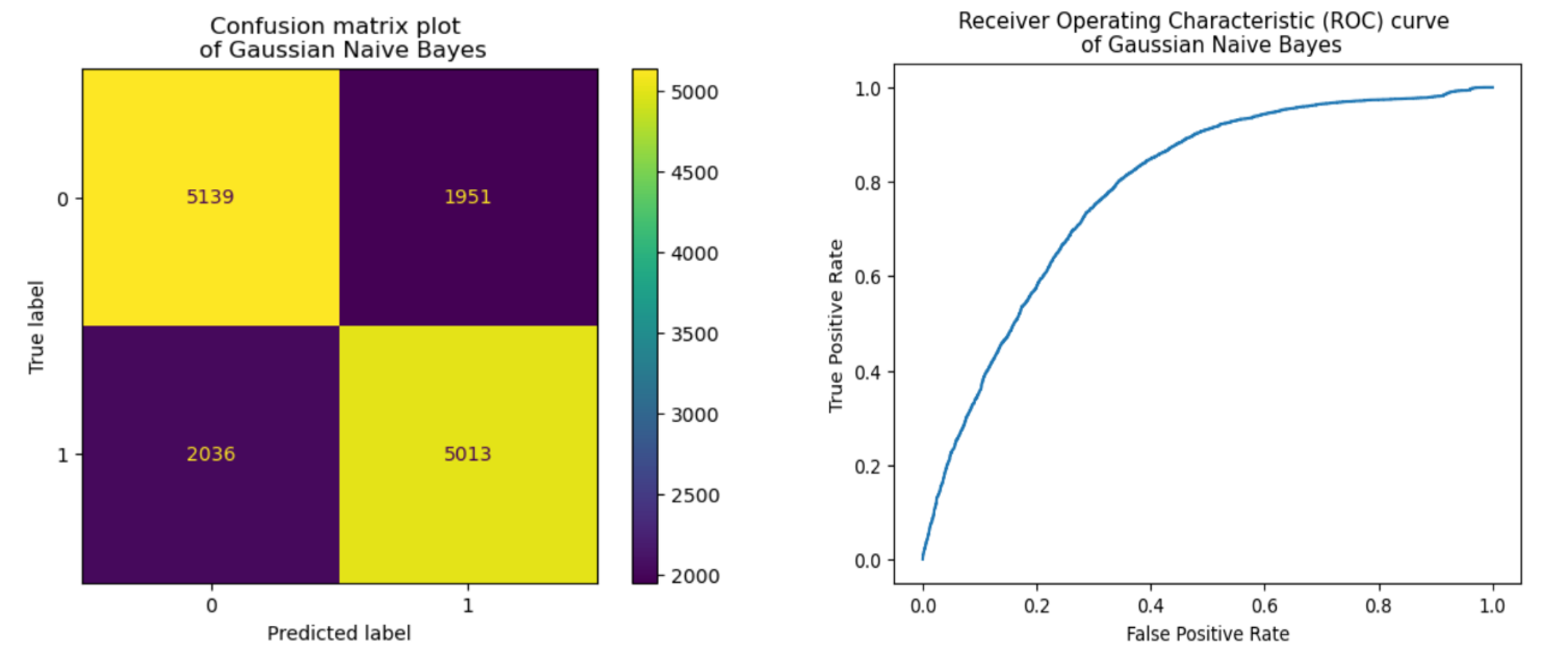
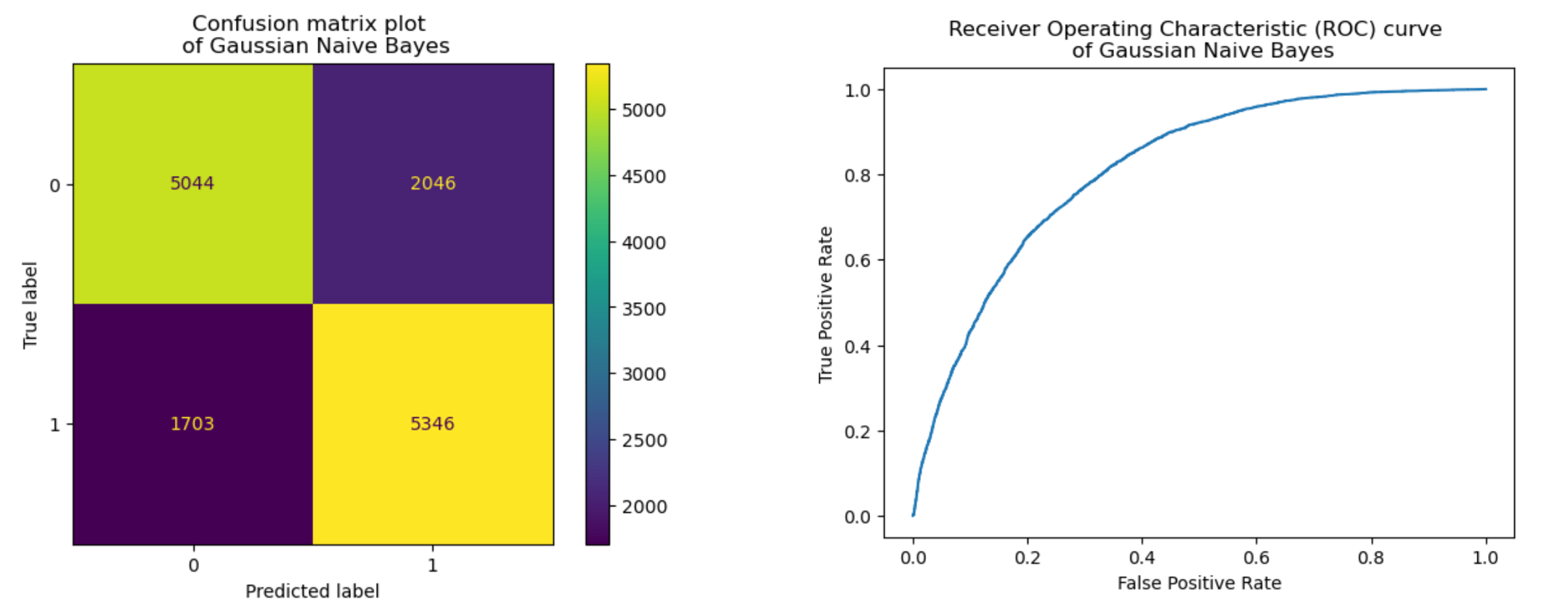
We decided to use the Gaussian Naïve Bayes method since our balanced diabetes dataset features normalized attributes ranging from 0 to 1 as continuous numbers. This method assumes that the distribution of each feature follows a Gaussian probability density function (PDF). We trained and tested the model using an 80-20 split of the dataset and applying different dimensionality reduction techniques. Below we show a summary of the obtained results:
| Mertrics | Normal | PCA 90% | PCA 95% | Forward feature selected dataset |
|---|---|---|---|---|
| Sensitivity: | 0.711 | 0.655 | 0.638 | 0.758 |
| Specificity: | 0.725 | 0.71 | 0.732 | 0.711 |
| Accuracy: | 0.718 | 0.683 | 0.685 | 0.735 |
| Precision: | 0.72 | 0.692 | 0.703 | 0.723 |
| Recall: | 0.711 | 0.655 | 0.638 | 0.758 |
| F1-score: | 0.715 | 0.673 | 0.669 | 0.74 |
| AROC: | 0.718 | 0.683 | 0.685 | 0.735 |
As our dataset is balanced, the value of accuracy, precision, recall and F1 score are similar and can all be used to represent the performance of our model. From the table above, the data is processed from the normal, scaled dataset in 3 different ways, first is PCA with 90% variance, second is PCA with 95% variance, and finally, forward feature selection using the SequentialFeatureSelector from mlxtend library with 5-fold cross-validation. The Forward feature selected dataset has 7 Features that provide the highest prediction accuracy including HighBP, HighChol, BMI, GenHlth, Sex, Age, Income.
As you can see from the table, the data with both PCA variations have, on average, lower performance than the normal scaled dataset while the Forward feature selected dataset performs better than any other dataset. The additional plots below visualize the confusion matrix and Receiver Operating Characteristics (ROC) curve from the normal scaled dataset and Forward feature selected dataset with 7 most important features.
K-Nearest Neighbors (KNN)
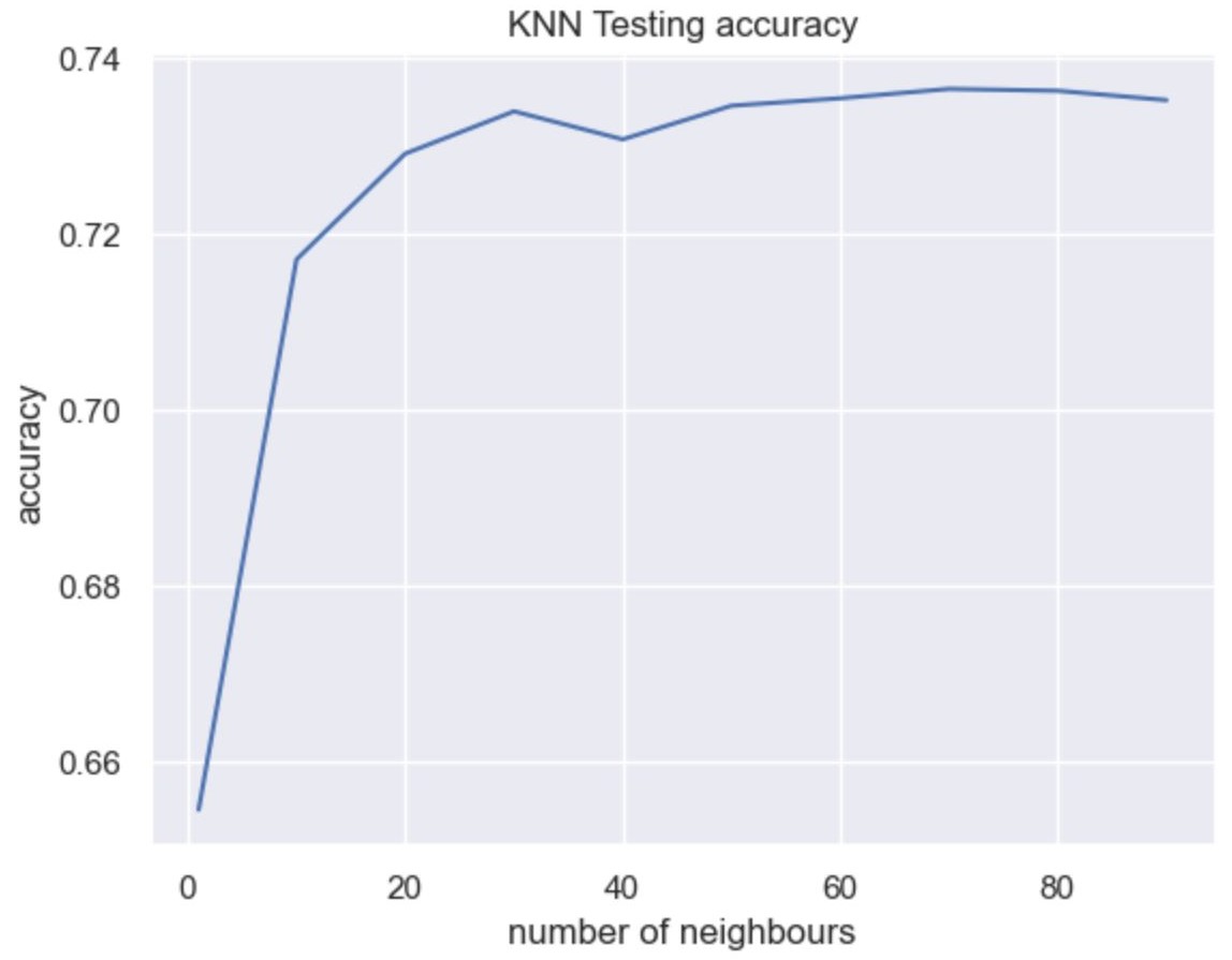
we also employed the K-Nearest Neighbors (KNN) method. In KNN classification, a class label is assigned based on a majority vote, meaning that the most frequent label among a given data point's neighbors is used. In our case, we utilized scikit-learn's KNeighborsClassifier to develop the KNN algorithm for binary classification. We separated the labels and features in the dataset and applied the KNN algorithm to the training split.
Since the optimal number of neighbors was unknown, we employed GridSearchCV to identify the best value. The optimal value was found to be 70 neighbors. With this configuration, we achieved an accuracy of 73.64% for the testing data. The graph below provides a visual representation of the results.
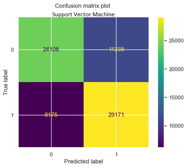
Support Vector Machine (SVM)
We have implemented the Support Vector Machine (SVM) method of supervised learning using default parameters in the scikit-learn package. This approach yielded an accuracy of 76.45%. To enhance the model, we are in the process of optimizing parameters further.
We have experimented with various kernels, such as the Radial Basis Function (RBF) kernel, which is popular due to its similarity to the KNN algorithm. By iterating over different C values, we achieved a maximum accuracy of 75.37%. We are continuing our efforts to improve the model's performance. Currently, each iteration requires approximately one hour of training time.
| Metric | Value |
|---|---|
| Sensitivity | 0.825 |
| Specificity | 0.682 |
| Accuracy | 0.754 |
| Precision | 0.722 |
| Recall | 0.825 |
| F1-score | 0.77 |
| AROC | 0.754 |
To further improve the accuracy of the SVM algorithm, we performed hyperparameter tuning by iterating between different C and gamma values in the range of C from 0.1 to 20 and gamma values of 0.1 and 0.001. However, despite trying different combinations of hyperparameters, we could not observe significant improvement in the accuracy values, which remained around 75%.
To overcome the challenge of dealing with high-dimensional data, we attempted to improve the accuracy of the SVM algorithm by using embedded autoencoders. Autoencoders are neural networks that can be used for unsupervised dimensionality reduction by learning a compressed representation of the input data. By reducing the dimensions of the features, we hoped to address the curse of dimensionality and improve the performance of the SVM algorithm. The image below shows a particular architecture that had a 1% value loss over 50 epochs. Encouraged by these results, we passed the encoded data to the SVM and evaluated the performance on both the training and testing datasets. However, the improvement in accuracy was only marginal, with the model achieving 78% accuracy on the training data and 71% accuracy on the testing data. While the use of autoencoders can help to address the issue of high dimensionality, the effectiveness of this approach is highly dependent on the architecture of the autoencoder and the complexity of the data. Further experimentation and tuning may be necessary to achieve significant improvements in the accuracy of the SVM algorithm.

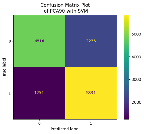
Finally, to attempt reducing the dimensionality of the data again and improve the efficiency of the model, we used the data after performing PCA analysis. We tested the model's performance using both 95% PCA data and 90% PCA data, and found that both sets of reduced features achieved an accuracy of 75.36% on the training data and 75.32% on the testing data.
| Metric | Value |
|---|---|
| Sensitivity | 0.823 |
| Specificity | 0.683 |
| Accuracy | 0.753 |
| Precision | 0.723 |
| Recall | 0.825 |
| F1-score | 0.77 |
| AROC | 0.753 |
Neural Networks (NN)
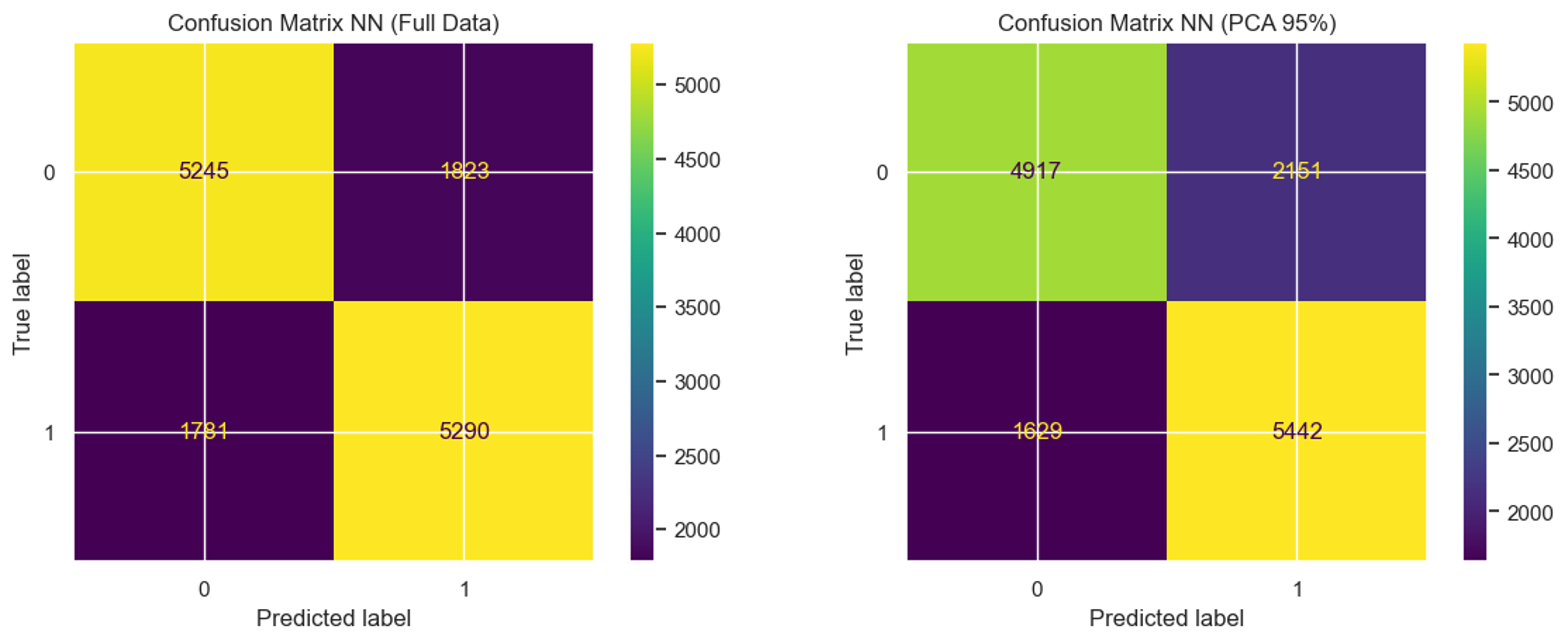
We implemented two versions of neural network-based classification to improve the accuracy of our model. The first version was trained on a balanced dataset with both the data and labels included. The second version was trained on a reduced dataset that was preprocessed using Principal Component Analysis (PCA) with 95% variance. Both models had similar structures with deep hidden layers and regularization layers added wherever necessary. The structure of the neural networks is shown in the figure below. This approach allowed us to compare the performance of the neural network model with and without dimensionality reduction, and determine the optimal approach for our classification problem.

To prevent overfitting and improve the performance of the neural network-based classification model, we implemented L2 regularization with a coefficient of 0.001 for all three layers. In addition, we included Dropout layers with a value of 0.2 to further prevent overfitting. Without these regularization techniques, we observed high training accuracy and lower validation accuracy.
For classification, we used the binary_crossentropy loss function and the Adam optimizer. The learning rate was set to 0.001 initially, and started decaying with a factor of 0.99 after 1000 epochs. The batch size was set to 128 to improve the efficiency of the training process.
We evaluated the performance of the model with and without PCA dimensionality reduction. Surprisingly, the model trained on the full dataset with regularization achieved an accuracy of 0.7523, while the model trained on the reduced PCA components achieved a lower accuracy of 0.7327. We also generated confusion matrices for both runs to better understand the performance of the model on the test data. These results suggest that while regularization techniques can help to improve the performance of neural network-based models, the effectiveness of PCA for dimensionality reduction may depend on the specific characteristics of the data.
We can see a greater number of false positives in both test cases, although the accuracy might be low, the false positives might indicate people that they need to take care of themselves to prevent diabetes.
| Metric | Value |
|---|---|
| Accuracy | 0.7523 |
| Precision | 0.7481 |
| Recall | 0.7437 |
| F1-score | 0.7459 |
| AROC | 0.7451 |
| Metric | Value |
|---|---|
| Accuracy | 0.7326 |
| Precision | 0.7696 |
| Recall | 0.7167 |
| F1-score | 0.7422 |
| AROC | 0.7339 |
Conclusions and Next Steps
The PCA analysis did not yield sufficient insights regarding specific features that may be less important for training our models. Additionally, we noted that certain variables, such as having a healthcare package, exhibited weak correlations with the presence of diabetes. As a result, we employed the alternative feature selection techniques of forward feature selection, to gain a more comprehensive understanding of each feature's impact on the performance of our classification models.
The supervised learning model methods were tested with the full feature dataset, PCA-applied dataset with 90% and 95% variance, and forward feature selection. The models were evaluated using multiple metrics, with a priority on reducing False-negative predictions to avoid missing patients with potential diabetes, given that our dataset and objective are focused on disease prediction, hence, False-positive is not as severe as False-negative. As a result, the metrics we will use to compare between models are accuracy, recall, and AROC.
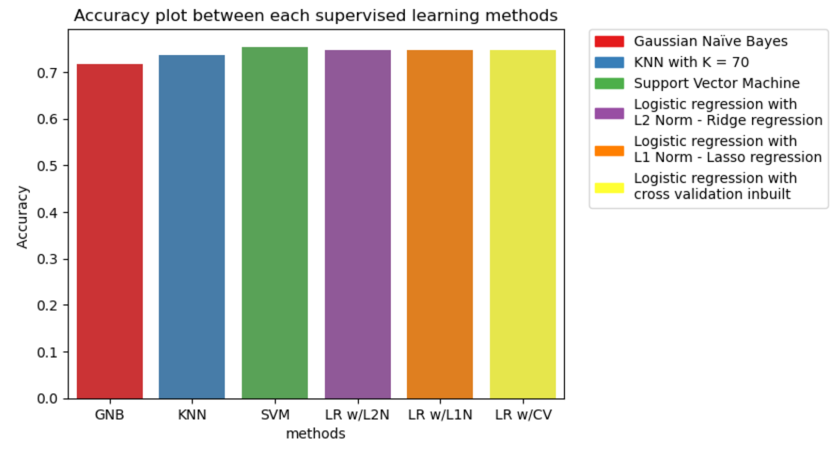
The comparison plot of accuracy, recall, and AROC is shown below. The model with the best performance in terms of accuracy, recall, and AROC is the Support Vector Machine (SVM) with an RBF kernel. Therefore, it is the most suitable model for achieving our objective of diabetes prediction.
Contribution Table
| Team Member | GitHub Page | Data Analysis and Preprocessing | Logistic Regression | SVM | KNN and NN | Naïve Bayes | Midterm Report Writting |
|---|---|---|---|---|---|---|---|
| Pranathi Suresha | |||||||
| Thanapol Tantagunninat | |||||||
| Chaitanya Mehta | |||||||
| Kanishk . | |||||||
| Juan Antonio Robledo |
References
- Diabetes Health Indicators Dataset [Internet]. [cited 2023 Feb 17]. Available from: https://www.kaggle.com/datasets/alexteboul/diabetes- health-indicators-dataset
- Behavioral Risk Factor Surveillance System [Internet]. [cited 2023 Feb 17]. Available from: https://www.kaggle.com /datasets/cdc/behavioral-risk-factor-surveillance-system
- Choubey DK, Kumar P, Tripathi S, Kumar S. Performance evaluation of classification methods with PCA and PSO for diabetes. Netw Model Anal Health Inform Bioinforma. 2020 Dec;9(1):5.
- Hasan MdK, Alam MdA, Das D, Hossain E, Hasan M. Diabetes Prediction Using Ensembling of Different Machine Learning Classifiers. IEEE Access. 2020;8:76516–31.
- Pima Indians Diabetes Database [Internet]. [cited 2023 Feb 23]. Available from: https://www.kaggle.com/ datasets/uciml/pima-indians-diabetes-database
- Xie Z, Nikolayeva O, Luo J, Li D. Building Risk Prediction Models for Type 2 Diabetes Using Machine Learning Techniques. Prev Chronic Dis. 2019 Sep 19;16: 190109.